Process methods

Calculators

derivesalinity

RSK.derivesalinity(seawaterLibrary: str = 'TEOS-10') → None

Calculate practical salinity.

Parameters:

seawaterLibrary (str, optional) – which underlying library this method should utilize. Current support includes: “TEOS-10”. Defaults to “TEOS-10”.

Calculates salinity from measurements of conductivity, temperature, and sea pressure, using the TEOS-10 GSW function gsw_SP_from_C. The result is added to the RSK.data field of the current RSK instance, and metadata in RSK.channels is updated. It requires the current RSK instance to be populated with conductivity, temperature, and pressure data.

If there is already a salinity channel present, this method replaces the values with a new calculation of salinity.

If sea pressure is not present, this method calculates it with the default atmospheric pressure, usually 10.1325 dbar. We suggest using RSK.deriveseapressure() before this for customizable atmospheric pressure.

Example:

>>> rsk.derivesalinity()
... # Optional arguments
... rsk.derivesalinity(seawaterLibrary="TEOS-10")

deriveseapressure

RSK.deriveseapressure(patm: Optional[Union[float, Collection[float]]] = None) → None

Calculate sea pressure.

Parameters:

patm (Union[float, Collection[float]], optional) – atmosphere pressure for calculating the sea pressure. Defaults to None (see below).

Calculates sea pressure from pressure and atmospheric pressure. The result is added to the RSK.data field of the current RSK instance, and metadata in RSK.channels is updated. It requires the current RSK instance to be populated with pressure data.

The patm argument is the atmospheric pressure used to calculate the sea pressure. A custom value can be used; otherwise, the default is to retrieve the value stored in the parameters field or to assume it is 10.1325 dbar if the parameters field is unavailable. This method also supports a variable patm input as a list, when that happens, the input list should have the same length as RSK.data.

If there is already a sea pressure channel present, the function replaces the values with the new calculation of sea pressure based on the values currently in the pressure column.

Example:

>>> rsk.deriveseapressure()
... # Optional arguments
... rsk.deriveseapressure(patm=10.1)

derivedepth

RSK.derivedepth(latitude: float = 45.0, seawaterLibrary: str = 'TEOS-10') → None

Calculate depth from pressure.

Parameters:

• latitude (float, optional) – latitude of the pressure measurement in decimal degrees. Defaults to 45.0.

• seawaterLibrary (str, optional) – which underlying library this method should utilize. Current support includes: “TEOS-10”. Defaults to “TEOS-10”.

Calculates depth from pressure. The result is added to the RSK.data field of the current RSK instance, and metadata in RSK.channels is updated. If there is already a depth channel present, this method replaces the values with the new calculation of depth.

If sea pressure is not present in the current RSK instance, it is calculated with the default atmospheric pressure (10.1325 dbar) by RSK.deriveseapressure() before deriving salinity when a different value of atmospheric pressure is used.

Example:

>>> rsk.derivedepth()
... # Optional arguments
... rsk.derivedepth(latitude=45.34, seawaterLibrary="TEOS-10")

derivevelocity

RSK.derivevelocity(windowLength: int = 3) → None

Calculate velocity from depth and time.

Parameters:

windowLength (int, optional) – length of the filter window used for the reference salinity. Defaults to 3.

Calculates profiling velocity from depth and time. The result is added to the RSK.data field of the current RSK instance, and metadata in RSK.channels is updated. It requires the current RSK instance to be populated with depth (see RSK.derivedepth()). The depth channel is smoothed with a running average of length windowLength to reduce noise, and then the smoothed depth is differentiated with respect to time to obtain a profiling speed.

If there is already a velocity channel present, this method replaces the velocity values with the new calculation.

If there is not a velocity channel but depth is present, this method adds the velocity channel metadata to RSK.channels and calculates velocity based on the values in the depth column.

Example:

>>> rsk.derivevelocity()
... # Optional arguments
... rsk.derivevelocity(windowLength=5)

deriveC25

RSK.deriveC25(alpha: float = 0.0191) → None

Calculate specific conductivity at 25 degrees Celsius in units of mS/cm.

Parameters:

alpha (float, optional) – temperature sensitivity coefficient. Defaults to 0.0191 deg C⁻¹.

Computes the specific conductivity in µS/cm at 25 degrees Celsius given the conductivity in mS/cm and temperature in degrees Celsius. The result is added to the RSK.data field of the current RSK instance, and metadata in RSK.channels is updated.

The calculation uses the Standard Methods for the Examination of Water and Waste Water (eds. Clesceri et. al.), 20th edition, 1998. The default temperature sensitivity coefficient, alpha, is 0.0191 deg C-1. Considering that the coefficient can range depending on the ionic composition of the water. The coefficient is made customizable.

Example:

>>> rsk.deriveC25()
... # Optional arguments
... rsk.deriveC25(alpha=0.0191)

deriveBPR

RSK.deriveBPR() → None

Convert bottom pressure recorder frequencies to temperature and pressure using calibration coefficients.

Loggers with bottom pressure recorder (BPR) channels are equipped with a Paroscientific, Inc. pressure transducer. The logger records the temperature and pressure output frequencies from the transducer. RSK files of type full contain only the frequencies, whereas RSK files of type EPdesktop contain the transducer frequencies for pressure and temperature, as well as the derived pressure and temperature.

This method derives temperature and pressure from the transducer frequency channels for full files. It implements the calibration equations developed by Paroscientific, Inc. to derive pressure and temperature. Both results are added to the RSK.data field of the current RSK instance, and metadata in RSK.channels is updated.

Example:

>>> rsk.deriveBPR()

deriveO2

RSK.deriveO2(toDerive: str = "concentration", unit: str = "µmol/l")) → None

Derives dissolved oxygen concentration or saturation.

Parameters:

• toDerive (str, optional) – O2 variable to derive, should only be “saturation” or “concentration”. Defaults to “concentration”.

• unit (str, optional) – unit of derived O2 concentration, valid inputs include “µmol/l”, “ml/l”, or “mg/l”. Defaults to “µmol/l”. Only effective when toDerive is concentration.

Derives dissolved O2 concentration from measured dissolved O2 saturation using R.F. Weiss (1970), or conversely, derives dissolved O2 saturation from measured dissolved O2 concentration using Garcia and Gordon (1992). The result is added to the RSK.data field of the current RSK instance, and metadata in RSK.channels is updated.

References

• R.F. Weiss, The solubility of nitrogen, oxygen and argon in water and seawater, Deep-Sea Res., 17 (1970), pp. 721-735

• H.E. Garc, L.I. Gordon, Oxygen solubility in seawater: Better fitting equations, Limnol. Oceanogr., 37 (6) (1992), pp. 1307-1312

Example:

>>> rsk.deriveO2()
... # Optional arguments
... rsk.deriveO2(toDerive="saturation", unit="ml/l")

derivebuoyancy

RSK.derivebuoyancy(latitude: float = 45.0, seawaterLibrary: str = 'TEOS-10') → None

Calculate buoyancy frequency N^2 and stability E.

Parameters:

• latitude (float, optional) – latitude in decimal degrees north [-90 … +90]. Defaults to 45.0.

• seawaterLibrary (str, optional) – which underlying library this method should utilize. Current support includes: “TEOS-10”. Defaults to “TEOS-10”.

Derives buoyancy frequency and stability using the TEOS-10 GSW toolbox library. The result is added to the RSK.data field of the current RSK instance, and metadata in RSK.channels is updated.

Note

The Absolute Salinity anomaly is taken to be zero to simplify the calculation.

Example:

>>> rsk.derivebuoyancy()
... # Optional arguments
... rsk.derivebuoyancy(latitude=45.34)

derivesigma

RSK.derivesigma(latitude: Optional[Union[float, Collection[float]]] = None, longitude: Optional[Union[float, Collection[float]]] = None, seawaterLibrary: str = 'TEOS-10') → None

Calculate potential density anomaly.

Parameters:

• latitude (Union[float, Collection[float]], optional) – latitude(s) in decimal degrees north. Defaults to None.

• longitude (Union[float, Collection[float]], optional) – longitude(s) in decimal degrees east. Defaults to None.

• seawaterLibrary (str, optional) – which underlying library this method should utilize. Current support includes: “TEOS-10”. Defaults to “TEOS-10”.

Derives potential density anomaly using the TEOS-10 GSW toolbox library. The result is added to the RSK.data field of the current RSK instance, and metadata in RSK.channels is updated.

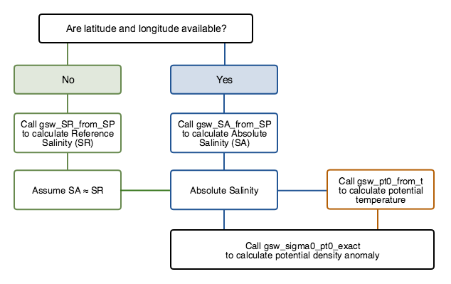
Note that this method also supports a variable latitude and longitude input as a list, when that happens, the input list should have the same length of RSK.data.

The workflow of the function is as below:

1. Calculate absolute salinity (SA)

   • When latitude and longitude data are available (from the optional input), this method will call SA = gsw_SA_from_SP(salinity,seapressure,lon,lat)

   • When latitude and longitude data are absent, this method will call SA = gsw_SR_from_SP(salinity) assuming that reference salinity equals absolute salinity approximately.

2. Calculate potential temperature pt0 = gsw_pt0_from_t(absolute salinity,temperature,seapressure)

3. Calculate potential density anomaly sigma0 = gsw_sigma0_pt0_exact(absolute salinity,potential temperature)

Example:

>>> rsk.derivesigma()
... # Optional arguments
... rsk.derivesigma(latitude=45.34, longitude=-75.91)

deriveSA

RSK.deriveSA(latitude: Optional[Union[float, Collection[float]]] = None, longitude: Optional[Union[float, Collection[float]]] = None, seawaterLibrary: str = 'TEOS-10') → None

Calculate absolute salinity.

Parameters:

• latitude (Union[float, Collection[float]]) – latitude(s) in decimal degrees north. Defaults to None.

• longitude (Union[float, Collection[float]]) – longitude(s) in decimal degrees east. Defaults to None.

• seawaterLibrary (str, optional) – which underlying library this method should utilize. Current support includes: “TEOS-10”. Defaults to “TEOS-10”.

Derives absolute salinity using the TEOS-10 GSW toolbox. The result is added to the RSK.data field of the current RSK instance, and metadata in RSK.channels is updated. The workflow of the function depends on if GPS information is available:

1. When latitude and longitude data are available (from the optional input), this method will call SA = gsw_SA_from_SP(salinity,seapressure,lon,lat)

2. When latitude and longitude data are absent, this method will call SA = gsw_SR_from_SP(salinity) assuming that reference salinity equals absolute salinity approximately.

Note

The latitude/longitude input must be either a single value or a list with the same length of RSK.data.

Example:

>>> rsk.deriveSA()
... # Optional arguments
... rsk.deriveSA(latitude=45.34, longitude=-75.91)

derivetheta

RSK.derivetheta(latitude: Optional[Union[float, Collection[float]]] = None, longitude: Optional[Union[float, Collection[float]]] = None, seawaterLibrary: str = 'TEOS-10') → None

Calculate potential temperature with a reference sea pressure of zero.

Parameters:

• latitude (Union[float, Collection[float]]) – latitude(s) in decimal degrees north. Defaults to None.

• longitude (Union[float, Collection[float]]) – longitude(s) in decimal degrees east. Defaults to None.

• seawaterLibrary (str, optional) – which underlying library this method should utilize. Current support includes: “TEOS-10”. Defaults to “TEOS-10”.

Derives potential temperature using the TEOS-10 GSW toolbox library. The result is added to the RSK.data field of the current RSK instance, and metadata in RSK.channels is updated. The workflow of this method is as below:

1. Calculate absolute salinity (SA)

   • When latitude and longitude data are available (from the optional input), this method will call SA = gsw_SA_from_SP(salinity,seapressure,lon,lat)

   • When latitude and longitude data are absent, this method will call SA = gsw_SR_from_SP(salinity) assuming that reference salinity equals absolute salinity approximately.

2. Calculate potential temperature pt0 = gsw_pt0_from_t(absolute salinity,temperature,seapressure)

Note

The latitude/longitude input must be either a single value or a list with the same length of RSK.data.

Example:

>>> rsk.derivetheta()
... # Optional arguments
... rsk.derivetheta(latitude=45.34, longitude=-75.91)

derivesoundspeed

RSK.derivesoundspeed(soundSpeedAlgorithm: str = 'UNESCO') → None

Calculate the speed of sound.

Parameters:

soundSpeedAlgorithm (str, optional) – algorithm to use, with the option of “UNESCO”, “DelGrosso”, or “Wilson”. Defaults to “UNESCO”.

Computes the speed of sound using temperature, salinity and pressure data. It provides three methods: UNESCO (Chen and Millero), Del Grosso, and Wilson, among which UNESCO is the default. The result is added to the RSK.data field of the current RSK instance, and metadata in RSK.channels is updated.

References

• C-T. Chen and F.J. Millero, Speed of sound in seawater at high pressures (1977) J. Acoust. Soc. Am. 62(5) pp 1129-1135

• V.A. Del Grosso, New equation for the speed of sound in natural waters (with comparisons to other equations) (1974) J. Acoust. Soc. Am 56(4) pp 1084-1091

• 23. 4. Wilson, Equations for the computation of the speed of sound in sea water, Naval Ordnance Report 6906, US Naval Ordnance Laboratory, White Oak, Maryland, 1962.

Example:

>>> rsk.derivesoundspeed()
... # Optional arguments
... rsk.derivesoundspeed(soundSpeedAlgorithm="DelGrosso")

deriveA0A

RSK.deriveA0A() → None

Apply the RBRquartz³ BPR|zero internal barometer readings to correct for drift in the marine Digiquartz pressure readings using the A-zero-A method.

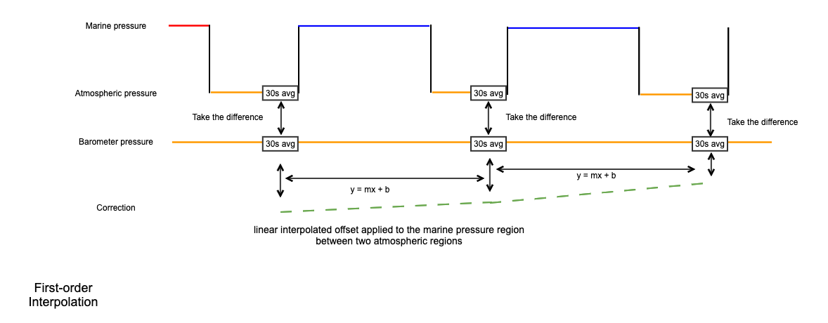
Uses the A-zero-A technique to correct drift in the Digiquartz® pressure gauge(s). This is done by periodically switching the applied pressure that the gauge measures from seawater to the atmospheric conditions inside the housing. The drift in quartz sensors is proportional to the full-scale rating, so a reference barometer - with hundreds of times less drift than the marine gauge - is used to determine the behaviour of the marine pressure measurements. The result is added to the RSK.data field of the current RSK instance, and metadata in RSK.channels is updated.

The A-zero-A technique, as implemented in this method, works as follows. The barometer pressure and the Digiquartz® pressure(s) are averaged over the last 30 s of each internal pressure calibration cycle. Using the final 30 s ensures that the transient portion observed after the valve switches is not included in the drift calculation. The averaged Digiquartz® pressure(s) are subtracted from the averaged barometer pressure, and these values are linearly interpolated onto the original timestamps to form the pressure correction. The drift-corrected pressure is the sum of the measured Digiquartz® pressure plus the drift correction.

Example:

>>> rsk.deriveA0A()

deriveAPT

RSK.deriveAPT(Alignment_coefficients: Collection[float] = None, Temperature_coefficients: Collection[float] = None, Acceleration_coefficients: Collection[float] = None) → None

Convert APT accelerations period and temperature period into accelerations and temperature.

The RBRquartz³ APT is a combined triaxial quartz accelerometer and a bottom pressure recorder. It is equipped with a Paroscientific, Inc. triaxial accelerometer and records the acceleration output frequencies from the accelerometer. Both ‘full’ and ‘EPdesktop’ RSK files contain only frequencies for acceleration and temperature.

This method derives 3-axis accelerations from the accelerometer frequency channels. It implements the calibration equations developed by Paroscientific, Inc. to derive accelerations. It requires users to input the alignment, temperature and acceleration coefficients. The coefficients are available on the Paroscientific, Inc. triax accelerometer instrument configuration sheet, which is shipped along with the logger. Derived accelerations and temperature are added to the RSK.data field of the current RSK instance, and the metadata in RSK.channels is updated.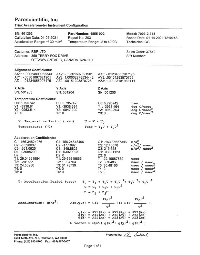

Example:

>>> Alignment_coefficients = [
...         [1.00024800955343, -0.00361697821901, -0.01234855907175],
...         [-0.00361697821901, 1.0000227853442, -0.00151293870726],
...         [-0.01234855907175, 0.00151293870726, 1.00023181988111],
...     ]
... Temperature_coefficients = [
...         [5.795742, 5.795742, 5.795742],
...         [-3938.81, -3938.684, -3938.464],
...         [-9953.514, -9947.209, -9962.304],
...         [0, 0, 0]
...     ]
... Acceleration_coefficients = [
...         [166.34824076, 156.24548496, -163.35657396],
...         [-5.328037,    -17.1992,     12.40078],
...         [-261.0626,    -342.8823,    215.658],
...         [0.03088299,   0.03029925,   0.03331123],
...         [0,            0,            0],
...         [29.04551984,  29.65519865,  29.19887879],
...         [-0.291685,    1.094704,     0.276486],
...         [24.50986,     31.78739,     30.48166],
...         [0,            0,            0],
...         [0,            0,            0],
...     ]
... rsk.deriveAPT(Alignment_coefficients, Temperature_coefficients, Acceleration_coefficients)

Post-processors

calculateCTlag

RSK.calculateCTlag(seapressureRange: Optional[Tuple[float, float]] = None, profiles: Optional[Union[int, Collection[int]]] = [], direction: str = 'both', windowLength: int = 21) → List[float]

Calculate a conductivity lag.

Parameters:

• seapressureRange (Tuple[float, float], optional) – limits of the sea_pressure range used to obtain the lag. Specify as a two-element tuple, [seapressureMin, seapressureMax]. Default is None ((0, max(seapressure))).

• profiles (Union[int, Collection[int]], optional) – profile number(s). Defaults to None (all available profiles)

• direction (str, optional) – cast direction of either “up”, “down”, or “both”. Defaults to “both”.

• windowLength (int, optional) – length of the filter window used for the reference salinity. Defaults to 21.

Returns:

List[float] – optimal lag of conductivity for each profile. These can serve as inputs into RSK.alignchannel().

Estimates the optimal conductivity time shift relative to temperature in order to minimise salinity spiking. The algorithm works by computing the salinity for conductivity lags of -20 to 20 samples at 1 sample increments. The optimal lag is determined by constructing a high-pass filtered version of the salinity time series for every lag, and then computing the standard deviation of each. The optimal lag is the one that yields the smallest standard deviation.

The seapressureRange argument allows for the possibility of estimating the lag on specific sections of the profile. This can be useful when unreliable measurements near the surface are found to impact the optimal lag, or when the profiling speed is highly variable.

The lag output by this method is compatible with the lag input argument for RSK.alignchannel() when lag units is specified as samples in RSK.alignchannel().

Example:

>>> rsk.calculateCTlag(seapressureRange=[0, 1.0])
... # Optional arguments
... rsk.calculateCTlag(seapressureRange=[0, 1.0], profiles=1, direction="up", windowLength=23)

alignchannel

RSK.alignchannel(channel: str, lag: Union[float, Collection[float]], profiles: Optional[Union[int, Collection[int]]] = [], direction: str = 'both', shiftfill: str = 'zeroorderhold', lagunits: str = 'samples') → None

Align a channel using a specified lag.

Parameters:

• channel (str) – longName of the channel to align (e.g. temperature)

• lag (Union[float, Collection[float]]) – lag to apply to the channel, negative lag shifts the channel backwards in time (earlier), while a positive lag shifts the channel forward in time (later)

• profiles (Union[int, Collection[int]], optional) – profile number(s). Defaults to None (all available profiles)

• direction (str, optional) – cast direction of either “up”, “down”, or “both”. Defaults to “both”.

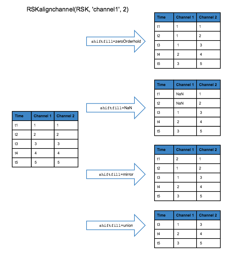
• shiftfill (str, optional) – shift fill treatment of “zeroorderhold”, “nan”, or “mirror”. Defaults to “zeroorderhold”.

• lagunits (str, optional) – lag units, either “samples” or “seconds”. Defaults to “samples”.

Shifts a channel in time by an integer number of samples or seconds in time, specified by the argument lag. A negative lag shifts the channel backwards in time (earlier), while a positive lag shifts the channel forward in time (later). Shifting a channel is most commonly used to align conductivity to temperature to minimize salinity spiking. It could also be used to adjust for the time delay caused by sensors with relatively slow adjustment times (e.g., dissolved oxygen sensors).

The shiftfill parameter describes what values will replace the shifted values. The default treatment is zeroorderhold, in which the first (or last) value is used to fill in the unknown data if the lag is positive (or negative). When shiftfill is nan, missing values are filled with NaNs. When shiftfill is mirror the edge values are mirrored to fill in the missing values. When shiftfill is union, all channels are truncated by lag samples. The diagram below illustrates the shiftfill options:

Example:

Using RSKalignchannel to minimize salinity spiking:

Salinity is derived with an empirical formula that requires measurements of conductivity, temperature, and pressure. The conductivity, temperature, and pressure sensors all have to be aligned in time and space to achieve salinity with the highest possible accuracy. Poorly-aligned conductivity and temperature data will result in salinity spikes in regions where the temperature and salinity gradients are strong. RSK.calculateCTlag() can be used to estimate the optimal lag by minimizing the spikes in the salinity time series, or the lag can be estimated by calculating the transit time for water to pass from the conductivity sensor to the thermistor. RSK.alignchannel() can then be used to shift the conductivity channel by the desired lag, and then salinity needs to be recalculated using RSK.derivesalinity().

>>> with RSK("example.rsk") as rsk:
...    rsk.computeprofiles(profile=range(0,9), direction="down")
...    # 1. Shift temperature channel of the first four profiles with the same lag value.
...    rsk.alignchannel(channel="temperature", lag=2, profiles=range(0,3))
...    # 2. Shift oxygen channel of first 4 profiles with profile-specific lags.
...    rsk.alignchannel(channel="dissolved_o2_concentration", lag=[2,1,-1,0], profiles=range(0,3))
...    # 3. Shift conductivity channel from all downcasts with optimal lag calculated with calculateCTlag().
...    lag = rsk.calculateCTlag()
...    rsk.alignchannel(channel="conductivity", lag=lag)

binaverage

RSK.binaverage(profiles: Optional[Union[int, Collection[int]]] = [], direction: str = 'down', binBy: str = 'sea_pressure', binSize: Union[float, Collection[float]] = 1.0, boundary: Union[float, Collection[float]] = []) → npt.NDArray

Average the profile data by a quantized reference channel.

Parameters:

• profiles (Union[int, Collection[int]], optional) – profile number(s). Defaults to None (all available profiles)

• direction (str, optional) – cast direction of either “up” or “down”. Defaults to “down”.

• binBy (str, optional) – reference channel that determines the samples in each bin, can be timestamp or any channel. Defaults to “sea_pressure”.

• binSize (Union[float, Collection[float]], optional) – size of bins in each regime. Defaults to 1.0, denoting 1 unit of binBy channel (e.g., 1 second when binBy is time).

• boundary (Union[float, Collection[float]], optional) – first boundary crossed in the direction selected of each regime, in the same units as binBy. Must have len(boundary) == len(binSize) or one greater. Defaults to [] (entire range).

Returns:

npt.NDArray – amount of samples in each bin.

Bins samples that fall within an interval and averages them, it is a form of data quantization. The bins are specified using two arguments: binSize and boundary.

1. binSize is the width (in units of binBy channel; i.e., meters if binned by depth) for each averaged bin. Typically the binSize should be a denominator of the space between boundaries, but if this is not the case, the new regime will start at the next boundary even if the last bin of the current regime is smaller than the determined binSize.

2. boundary determines the transition from one binSize to the next.

The cast direction establishes the bin boundaries and sizes. If the direction is up, the first boundary and binSize are closest to the seabed with the next boundaries following in descending order. If the direction is down, the first boundary and bin size are closest to the surface with the next boundaries following in descending order.

NOTE: The boundary takes precedence over the bin size. (Ex. boundary=[5.0, 20.0], binSize = [10.0 20.0]. The bin array will be [5.0 15.0 20.0 40.0 60.0…]). The default binSize is 1 dbar and the boundary is between minimum (rounded down) and maximum (rounded up) sea_pressure, i.e, [min(sea_pressure) max(sea_pressure)].

A common bin system is to use 1 dbar bins from 0.5 dbar to the maximum sea_pressure value. Here is the code and a diagram:

>>> rsk.binaverage(direction="down", binSize=1.0, boundary=0.5)

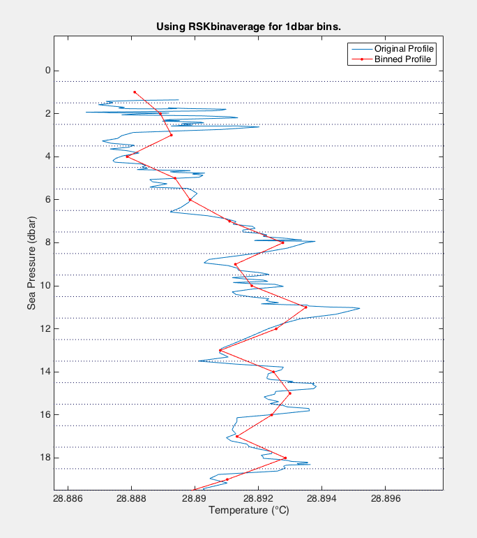
The figure above shows an original Temperature time series plotted against sea_pressure in blue. The dotted lines are the bin limits. The red dots are the averaged Temperature time series after being binned in 1dbar bins. The temperature values are centred in the middle of the bin (between the dotted lines) and are an average of all the values in the original time series that fall within the determined interval.

The diagram and code below describe the bin array for a more complex binning with different regimes throughout the water column:

>>> samplesinbin = rsk.binaverage(direction="down", binBy="Depth", binSize=[10.0, 50.0], boundary=[10.0, 50.0, 200.0])

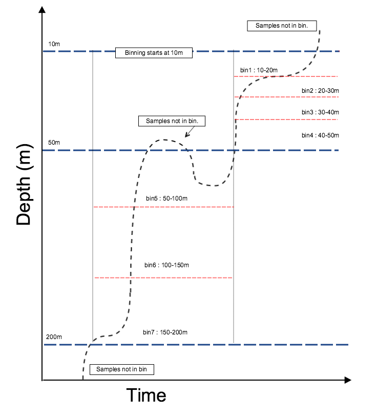
Note the discarded measurements in the image above the 50m dashed line. Once the samples have started in the next bin, the previous bin closes, and further samples in that bin are discarded.

The diagram and code below give an example when the average is done against time (i.e. binBy = “timestamp”), with the unit in seconds. Here we average for every ten minutes (i.e. 600 seconds).

>>> samplesinbin = rsk.binaverage(binBy="time", binSize=600.0)

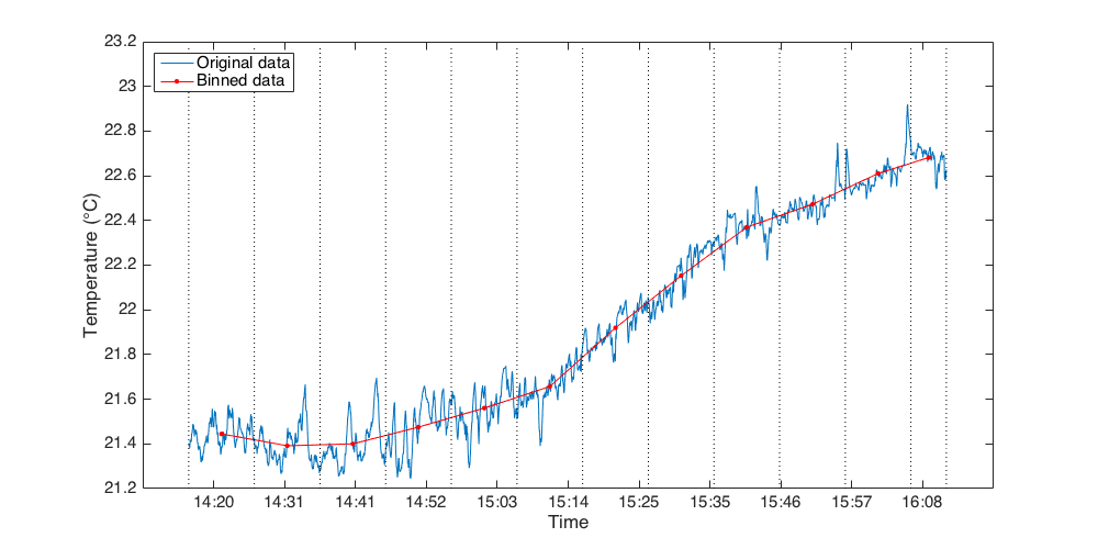
The figure above shows an original Temperature time series plotted against Time in blue. The dotted lines are the bin limits. The red dots are the averaged Temperature time series after being binned in 10 minutes bins. The temperature values are centred in the middle of the bin (between the dotted lines) and are an average of all the values in the original time series that fall within the determined interval.

correcthold

RSK.correcthold(channels: Union[str, Collection[str]] = [], profiles: Optional[Union[int, Collection[int]]] = [], direction: str = 'both', action: str = 'nan') → dict

Replace zero-order hold points with interpolated values or NaN.

Parameters:

• channels (Union[str, Collection[str]], optional) – longname of channel to correct the zero-order hold (e.g., temperature, salinity, etc). Defaults to [] (all available channels).

• profiles (Union[int, Collection[int]], optional) – profile number(s). Defaults to [] (all available profiles).

• direction (str, optional) – cast direction of either “up”, “down”, or “both”. Defaults to “both”.

• action (str, optional) – action to perform on a hold point. Given “nan”, hold points are replaced with NaN. Another option is “interp”, whereby hold points are replaced with values calculated by linearly interpolating from the neighbouring points. Defaults to “nan”.

Returns:

dict –

a reference dict with values giving the index of the corrected hold points; each returned key-value pair

has the channel name as the key and an array of indices relating to the respective channel as the value.

The analogue-to-digital (A2D) converter on RBR instruments must recalibrate periodically. In the time it takes for the calibration to finish, one or more samples are missed. The onboard firmware fills the missed sample with the same data measured during the previous sample, a simple technique called a zero-order hold.

This method identifies zero-hold points by looking for where consecutive differences for each channel are equal to zero and replaces them with an interpolated value or a NaN.

An example of where zero-order holds are important is when computing the vertical profiling rate from pressure. Zero-order hold points produce spikes in the profiling rate at regular intervals, which can cause the points to be flagged by RSK.removeloops().

Example:

>>> holdpts = rsk.correcthold()

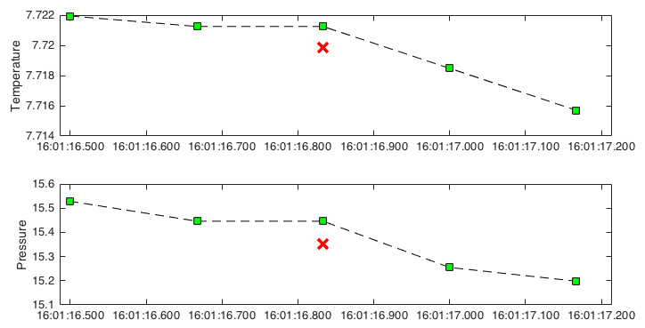
The green squares indicate the original data. The red crossings are the interpolated data after correcting zero-order holds.

despike

RSK.despike(channels: str, profiles: Optional[Union[int, Collection[int]]] = [], direction: str = 'both', threshold: int = 2, windowLength: int = 3, action: str = 'nan') → dict

Despike a time series on a specified channel.

Parameters:

• channels (str) – longname of channel to despike (e.g., temperature, or salinity, etc).

• profiles (Union[int, Collection[int]], optional) – profile number(s). Defaults to [] (all available profiles).

• direction (str, optional) – cast direction of either “up”, “down”, or “both”. Defaults to “both”.

• threshold (int, optional) – amount of standard deviations to use for the spike criterion. Defaults to 2.

• windowLength (int, optional) – total size of the filter window. Must be odd. Defaults to 3.

• action (str, optional) – action to perform on a spike. Given “nan”, spikes are replaced with NaN. Other options are “replace”, whereby spikes are replaced with the corresponding reference value, and “interp” whereby spikes are replaced with values calculated by linearly interpolating from the neighbouring points. Defaults to “nan”.

Returns:

dict – dict with values giving the index of the spikes.

Removes or replaces spikes in the data from the channel specified. The algorithm used here is to discard points that lie outside of a threshold. The data are smoothed by a median filter of length windowLength to produce a “reference” time series. Residuals are formed by subtracting the reference time series from the original time series. Residuals that fall outside of a threshold, specified as the number of standard deviations, where the standard deviation is computed from the residuals, are flagged for removal or replacement.

The default behaviour is to replace the flagged values with NaNs. Flagged values can also be replaced with reference values, or replaced with values linearly interpolated from neighbouring “good” values.

Example:

>>> spikes = rsk.despike(channel="Temperature", profiles=range(0, 4), direction="down",
        threshold=4.0, windowLength=11, action="nan")

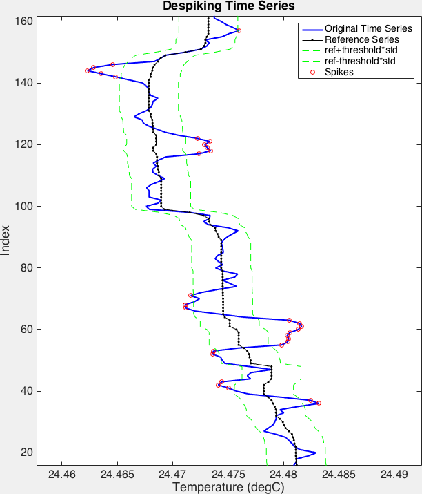
The red circles indicate the samples in the blue time series that spike. The green lines are the limits determined by the threshold parameter. The black time series is, as referred to above, the reference series. It is the filtered original time series.

smooth

RSK.smooth(channels: Union[str, Collection[str]], filter: str = 'boxcar', profiles: Optional[Union[int, Collection[int]]] = [], direction: str = 'both', windowLength: int = 3) → None

Apply a low pass filter on the specified channel(s).

Parameters:

• channels (Union[str, Collection[str]]) – longname of channel to filter. Can be a single channel, or a list of multiple channels.

• filter (str, optional) – the weighting function, “boxcar”, “triangle”, or “median”. Defaults to “boxcar”.

• profiles (Union[int, Collection[int]], optional) – profile number(s). Defaults to [] (all available profiles).

• direction (str, optional) – cast direction of either “up”, “down”, or “both”. Defaults to “both”.

• windowLength (int, optional) – the total size of the filter window. Must be odd. Defaults to 3.

Applies a low-pass filter to a specified channel or multiple channels with a running average or median. The sample being evaluated is always in the centre of the filtering window to avoid phase distortion. Edge effects are handled by mirroring the original time series.

The windowLength argument determines the degree of smoothing. If windowLength = 5; the filter is composed of two samples from either side of the evaluated sample and the sample itself. windowLength must be odd to centre the average value within the window.

The median filter is less sensitive to extremes (best for spike removal), whereas the boxcar and triangle filters are more effective at noise reduction and smoothing.

Example:

>>> rsk.smooth(channels=["temperature", "salinity"], windowLength=17)

The figures below demonstrate the effect of the different available filters:

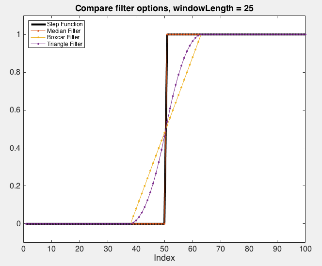
The effect of the various low-pass filters implemented by RSKsmooth() on a step function. Note that in this case, the median filter leaves the original step signal unchanged.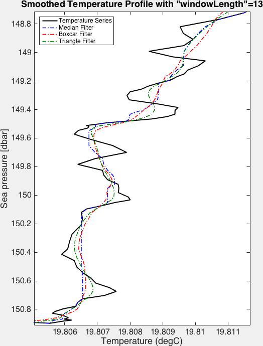

Example of the effect of various low-pass filters on a time series.

removeloops

RSK.removeloops(profiles: Optional[Union[int, Collection[int]]] = [], direction: str = 'both', threshold: float = 0.25) → List[int]

Remove data with a profiling rate less than a threshold and with reversed pressure (loops).

Parameters:

• profiles (Union[int, Collection[int]], optional) – profile number(s). Defaults to [] (all available profiles).

• direction (str, optional) – cast direction of either “up”, “down”, or “both”. Defaults to “both”.

• threshold (float, optional) – minimum speed at which the profile must be taken. Defaults to 0.25 m/s.

Returns:

dict – dict with values giving the index of the samples that are flagged

Flags and replaces pressure reversals or profiling slowdowns with NaNs in the data field of this RSK instance and returns the index of these samples. Variations in profiling rate are caused by, for example, profiling from a vessel in rough seas with a taut wire, or by lowering a CTD hand over hand. If the ship heave is large enough, the CTD can momentarily change direction even though the line is paying out, causing a “loop” in the velocity profile. Under these circumstances the data can be contaminated because the CTD samples its own wake; this method is designed to minimise the impact of such situations.

First, this method low-pass filters the depth channel with a 3-point running average boxcar window to reduce the effect of noise. Second, it calculates the velocity using a simple two-point finite difference scheme and interpolates the velocity back onto the original timestamps. Lastly, it flags samples associated with a profiling velocity below the threshold value and replaces the corresponding points in all channels with NaN. Additionally, any data points with reversed pressure (i.e. decreasing pressure during downcast or increasing pressure during upcast) will be flagged as well, to ensure that data with above threshold velocity in a reversed loop are removed.

The convention is for downcasts to have positive profiling velocity. This method automatically accounts for the upcast velocity sign change.

NOTE:

The input RSK must contain a depth channel. See RSK.derivedepth().

While the depth channel is filtered by a 3-point moving average in order to calculate the profiling velocity, the depth channel in the RSK.data is not altered.

Example:

>>> loops = rsk.removeloops(direction= "down", threshold= 0.1)

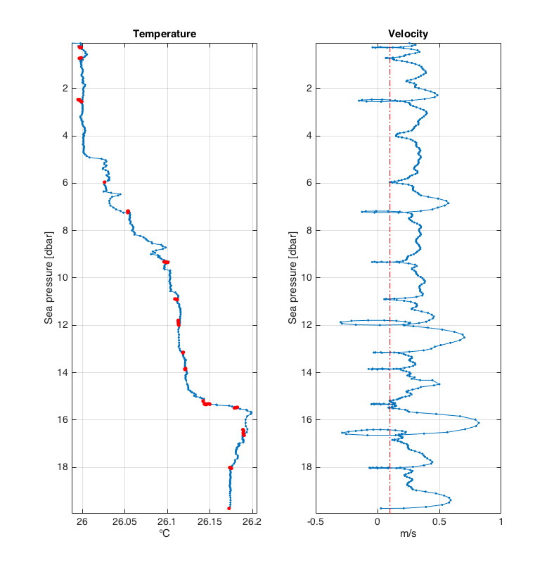
Shown here are profiles of temperature (left panel) and profiling velocity (right panel). The red dash-dot line illustrates the threshold velocity; set in this example to 0.1 m/s. The temperature readings for which the profiling velocity was below 0.1 m/s are illustrated by the red dots.

trim

RSK.trim(reference: str, range: Tuple[Union[np.datetime64, int], Union[np.datetime64, int]], channels: Union[str, Collection[str]] = [], profiles: Optional[Union[int, Collection[int]]] = [], direction: str = 'both', action: str = 'nan') → List[int]

Remove or replace values that fall in a certain range.

Parameters:

• reference (str) – channel that determines which samples will be in the range and trimmed. To trim according to time, use “time”, or, to trim by index, choose “index”.

• range (Tuple[Union[np.datetime64, int], Union[np.datetime64, int]]) – A 2-element tuple of minimum and maximum values. The samples in “reference” that fall within the range (including the edges) will be trimmed. If “reference” is “time”, then each range element must be a NumPy datetime64 object.

• channels (Union[str, Collection[str]]) – apply the flag to specified channels. When action is set to remove, specifying channel will not work. Defaults to [] (all available channels).

• profiles (Union[int, Collection[int]], optional) – profile number(s). Defaults to [] (all available profiles).

• direction (str, optional) – cast direction of either “up”, “down”, or “both”. Defaults to “both”.

• action (str, optional) – action to apply to the flagged values. Can be “nan”, “remove”, or “interp”. Defaults to “nan”.

Returns:

List[int] – a list containing the indices of the trimmed samples.

The reference argument could be a channel name (e.g. sea_pressure), time, or index. The range argument is a 2-element vector of minimum and maximum values. The samples in reference that fall within the range (including the edge) will be trimmed. When reference is time, each range element must be a np.datetime64 object. When reference is index, each range element must be an integer number.

This method provides three options to deal with flagged data, which are:

1. nan - replace flagged samples with NaN

2. remove - remove flagged samples

3. interp - replace flagged samples with interpolated values by neighbouring points.

Example:

>>> # Replace data acquired during a shallow surface soak with NaN
... rsk.trim(reference="sea_pressure", range=[-1.0, 1.0], action="NaN")
...
... # Remove data before 2022-01-01
... rsk.trim(reference="time", range=[np.datetime64("0"), np.datetime64("2022-01-01")], action="remove")

correctTM

RSK.correctTM(alpha: float, beta: float, gamma: float = 1.0, profiles: Optional[Union[int, Collection[int]]] = [], direction: str = 'both') → None

Apply a thermal mass correction to conductivity using the model of Lueck and Picklo (1990).

Args:

alpha (float): volume-weighted magnitude of the initial fluid thermal anomaly. beta (float): inverse relaxation time of the adjustment. gamma (float, optional): temperature coefficient of conductivity (dC/dT). Defaults to 1.0. profiles (Union[int, Collection[int]], optional): profile number(s). Defaults to [] (all available profiles). direction (str, optional): cast direction of either “up”, “down”, or “both”. Defaults to “both”.

Applies the algorithm developed by Lueck and Picklo (1990) to minimize the effect of conductivity cell thermal mass on measured conductivity. Conductivity cells exchange heat with the water as they travel through temperature gradients. The heat transfer changes the water temperature and hence the measured conductivity. This effect will impact the derived salinity and density in the form of sharp spikes and even a bias under certain conditions.

Example:

>>> rsk.correctTM(alpha=0.04, beta=0.1)

References

• Lueck, R. G., 1990: Thermal inertia of conductivity cells: Theory. J. Atmos. Oceanic Technol., 7, pp. 741 - 755. https://doi.org/10.1175/1520-0426(1990)007<0741:TIOCCT>2.0.CO;2

• Lueck, R. G. and J. J. Picklo, 1990: Thermal inertia of conductivity cells: Observations with a Sea-Bird cell. J. Atmos. Oceanic Technol., 7, pp. 756 - 768. https://doi.org/10.1175/1520-0426(1990)007<0756:TIOCCO>2.0.CO;2

correcttau

RSK.correcttau(channel: str, tauResponse: int, tauSmooth: int = 0, profiles: Optional[Union[int, Collection[int]]] = [], direction: str = 'both') → None

Apply tau correction and smoothing (optional) algorithm from Fozdar et al. (1985).

Parameters:

• channel (str) – longName of channel to apply tau correction (e.g., “Temperature”, “Dissolved O2”).

• tauResponse (int) – sensor time constant of the channel in seconds.

• tauSmooth (int, optional) – smoothing time scale in seconds. Defaults to 0.

• profiles (Union[int, Collection[int]], optional) – profile number(s). Defaults to [] (all available profiles).

• direction (str, optional) – cast direction of either “up”, “down”, or “both”. Defaults to “both”.

Sensors require a finite time to reach equilibrium with the ambient environment under variable conditions. The adjustment process alters both the magnitude and phase of the true signal. The time response of a sensor is often characterized by a time constant, which is defined as the time it takes for the measured signal to reach 63.2% of the difference between the initial and final values after a step change.

This method applies the Fozdar et al. (1985; Eq. 3.15) algorithm to correct the phase and response of a measured signal to more accurately represent the true signal. The Fozdar expression is different from others because it includes a smoothing time constant to reduce the noise added by sharpening algorithms. When the smoothing time constant is set to zero (the default value for RSK.correcttau()), the Fozdar algorithm reduces to the discrete form of a commonly-used model to correct for the thermal lag of a thermistor:

\[T = T_m + τ\frac{ dT_m }{ dt }\]

where \(T_m\) is the measured temperature, \(T\) is the true temperature, and τ is the thermistor time constant (Fofonoff et al., 1974).

Below is an example showing how the Fozdar algorithm, with no smoothing time constant, enhances the response of a RBRcoda T.ODO|standard (τ = 8s) data taken during a CTD profile. The CTD had an RBRcoda T.ODO|fast (τ = 1s) to serve as a reference. The graph shows that the Fozdar algorithm, when applied to data from the standard response optode, does a good job of reconstructing the true dissolved oxygen profile by recovering both the phase and amplitude lost by its relatively long time constant. The standard deviation of the difference between standard and fast optode is greatly reduced.

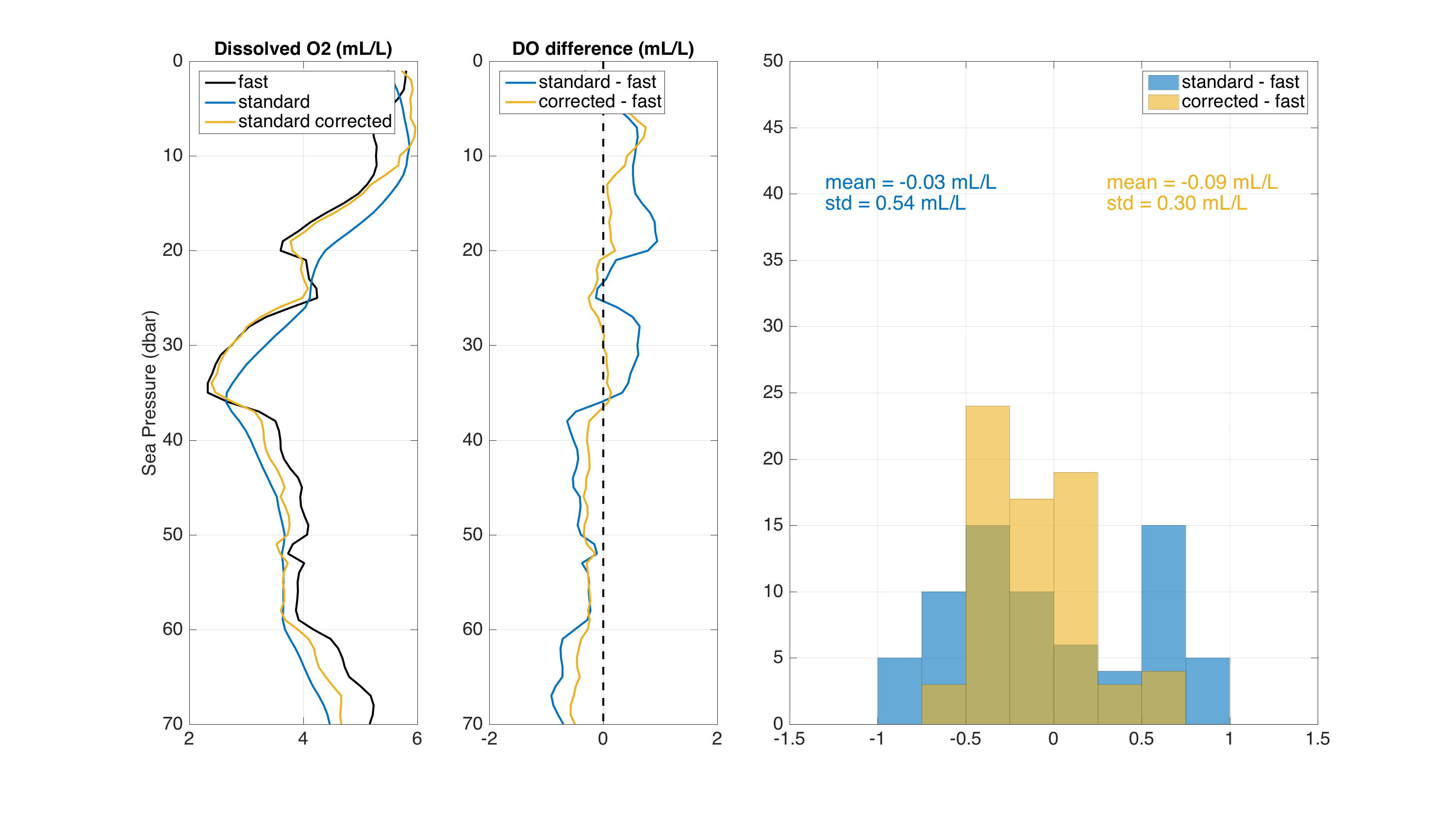
Dissolved O2 from T.ODO fast, T.ODO standard and T.ODO standard after tau correction (left panel) Dissolved O2 differences between T.ODO standard with and without correction and T.ODO fast (middle panel) Histogram of the differences (right panel).

The use of the Fozdar algorithm on RBR optode data is currently being studied at RBR, and more tests are needed to determine the optimal value for parameter tauSmooth on sensors with different time constants. RBR is also planning to evaluate the use of other algorithms that have been tested on oxygen optode data, such as the “bilinear” filter (Bittig et al., 2014).

Example:

>>> rsk.correcttau(channel="dissolved_o2_saturation", tauResponse=8, direction="down", profiles=1)

References

• Bittig, Henry C., Fiedler, Björn, Scholz, Roland, Krahmann, Gerd, Körtzinger, Arne, ( 2014), Time response of oxygen optodes on profiling platforms and its dependence on flow speed and temperature, Limnology and Oceanography: Methods, 12, doi: https://doi.org/10.4319/lom.2014.12.617.

• Fofonoff, N. P., S. P. Hayes, and R. C. Millard, 1974: WHOI/Brown CTD microprofiler: Methods of calibration and data handling. Woods Hole Oceanographic Institution Tech. Rep., 72 pp., https://doi.org/10.1575/1912/647.

• Fozdar, F.M., G.J. Parkar, and J. Imberger, 1985: Matching Temperature and Conductivity Sensor Response Characteristics. J. Phys. Oceanogr., 15, 1557-1569, https://doi.org/10.1175/1520-0485(1985)015<1557:MTACSR>2.0.CO;2.

generate2D

RSK.generate2D(channels: Union[str, Collection[str]] = [], profiles: Optional[Union[int, Collection[int]]] = [], direction: str = 'down', reference: str = 'sea_pressure') → Image

Generate data for 2D plot by RSK.images().

Parameters:

• channels (Union[str, Collection[str]], optional) – longName of channel(s) to generate data. Defaults to [] (all available channels).

• profiles (Union[int, Collection[int]] , optional) – profile numbers to use. Defaults to [] (all available profiles).

• direction (str, optional) – cast direction of either “up” or “down”. Defaults to “down”.

• reference (str, optional) – channel that will be used as y dimension. Defaults to “sea_pressure”.

Arranges a series of profiles from selected channels into in a 3D matrix. The matrix has dimensions MxNxP, where M is the number of depth or pressure levels, N is the number of profiles, and P is the number of channels. Arranged in this way, the matrices are useful for analysis and for 2D visualization (RSK.images() uses RSK.generate2D()). It may be particularly useful for users wishing to visualize multidimensional data without using RSK.images(). Each profile must be placed on a common reference grid before using this method (see RSK.binaverage()).

Example:

>>> rsk.generate2D(channels=["temperature", "conductivity"], direction="down")

centrebursttimestamp

RSK.centrebursttimestamp() → None

Modify wave/BPR file timestamp in the data field from beginning to middle of the burst.

For wave or BPR loggers, Ruskin stores the raw high-frequency values in the burstData field. The data field is composed of one sample for each burst with a timestamp set to be the first value of each burst period; the sample is the average of the values during the corresponding burst. For users’ convenience, this method modifies the timestamp from the beginning of each burst to the middle of it.

NOTE: This method examines if the rsk file contains burstData field, if not, it will not proceed.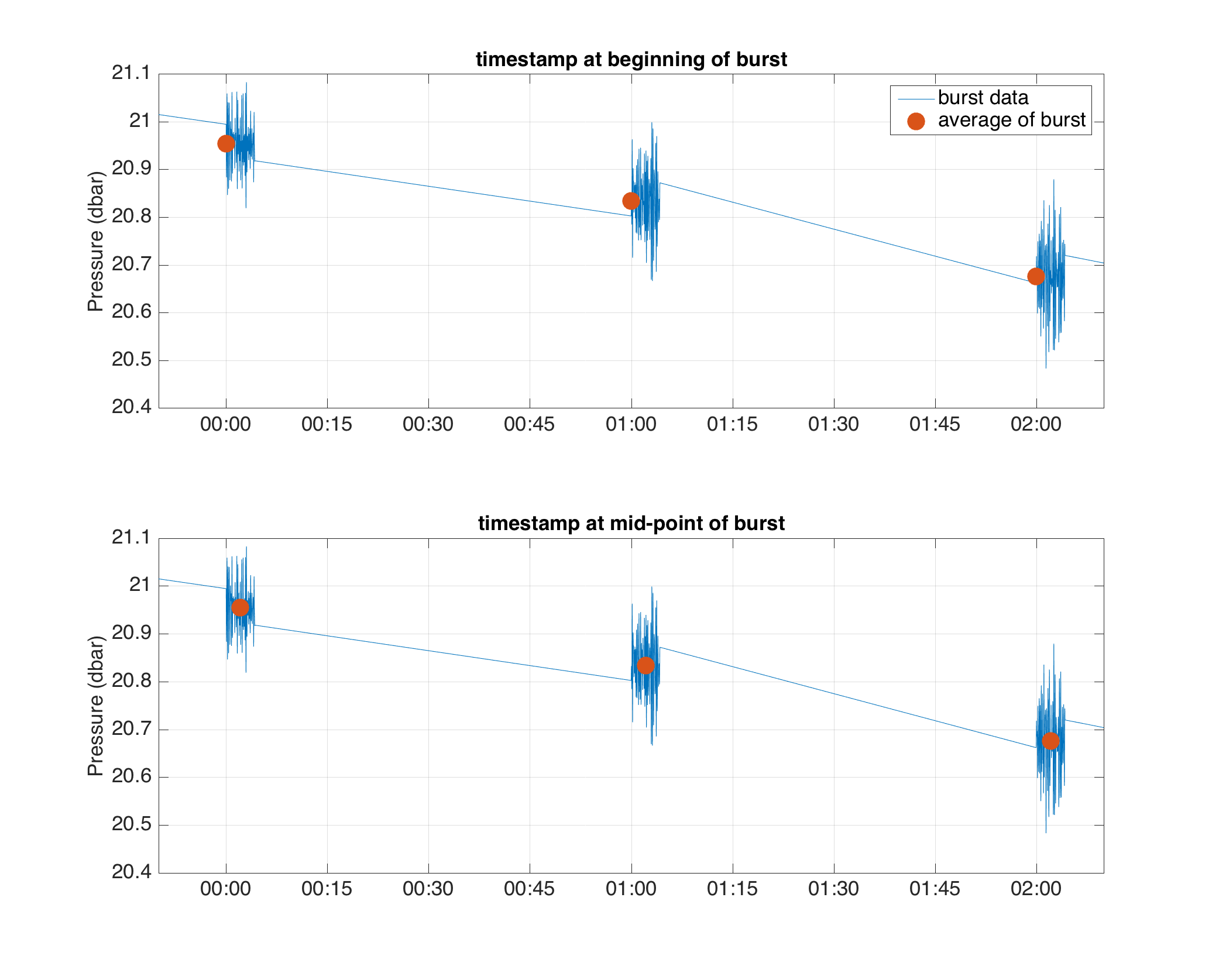

In the figure above, the blue line is the values in the burstdata field and the red dots are the values in the data field (i.e. the average of each burst period). The top panel shows the timestamp at beginning of the burst, while the bottom panel shows the timestamp in the middle of the burst after the application of this method.

Example:

>>> rsk.centrebursttimestamp()