Integrating with a profiling float

Introduction

There are a number of dedicated features in the Logger2 products aimed at profiling floats.  The primary requirement of these vehicles is to have multiple sampling regimes that are enabled according to depth.

The typical Argo profiler might be set up with the following behaviour:

 

Control of buoyancy

For the majority of this 10 day schedule, the RBR instrument is used purely as a depth sensor, providing input to the buoyancy engine and float controller.  This is typically done interactively using the fetch command, which can be performed at any time, regardless of whether the RBR instrument logging schedule is enabled or not.  The RBR will automatically fall asleep after an idle timeout of a few seconds, but in order to minimize the power consumption, it is recommended that the command fetch sleepafter = true is used.  This will override the idle timeouts and does not affect any ongoing deployment. In order to wake up the instrument, a <cr> character should precede any command.  This is a useful practice in any situation when it is not clear whether or not the instrument is asleep.

Setup for deployment

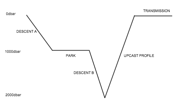
The real science of the Argo profiler occurs during the upcast, typically from 2000dbar to the surface.  For historical and scientific reasons, this is often a multi-stage ascent, where the sampling and binning requirements change according to depth. The expanded figure below shows an example of a typical ascent setup.

 

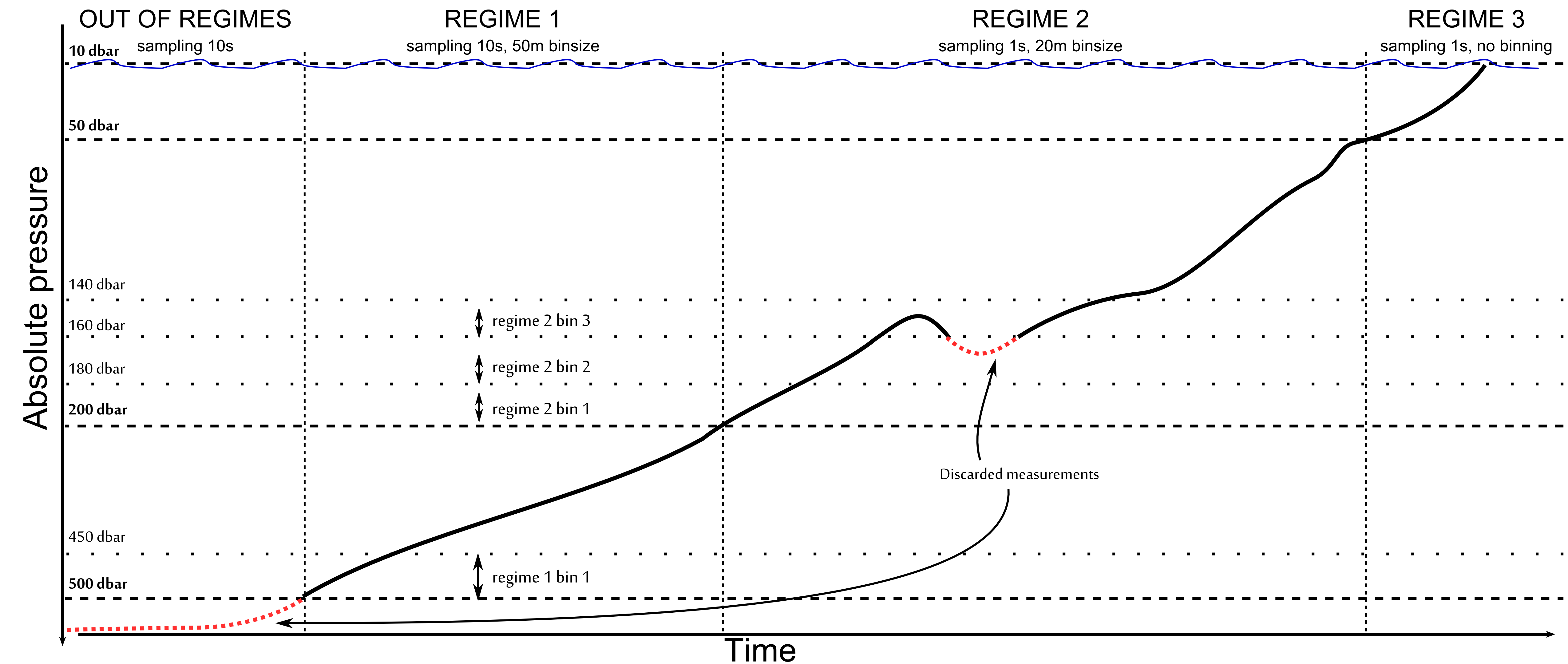
As is clear, there are three distinct sampling regimes that are required.  Each of them has a boundary, a sampling speed, and an averaging bin size.  

• The boundary determines when the regime comes into effect (dbar).
• The sampling speed dictates the measurement rate that is used internally (msec).
• The bin size dictates the amount of water column (in dbar) over which the samples will be averaged and stored.

To accomplish this task, a combination of the regimes and three regime commands are needed.

 

First, one should tell the logger that it will be ascending (decreasing water pressure) using three sampling regimes, and the absolute pressure serves as reference.

Configure the regime closest to the seabed (10s sampling rate, 50m bin, bottom boundary 500 dbar):Then the middle one (1s sampling rate, 20m bin, bottom boundary 200 dbar):Then the regime closest to the sea surface (1s sampling rate, no binning, bottom boundary 50 dbar):Finally put the logger in regimes mode:

With this setup, the logger will only start recording data once the boundary of the first regime is crossed.  In this example, if the RBR instrument is enabled while the float is at 700 dbar, then starts to ascend, no data will be stored until 500 dbar.  If the float is at 490 dbar when the RBR instrument is enabled, sampling will start immediately as the first regime is already in effect.

Instruments with firmware version 1.100 or later may also support a derived data channel, type cnt_00, which contains a count of the number of measurements in the averaged bin when in the regimes sampling mode. As with any other channel, it may be turned on or off as needed; see the channel command. The benefit of turning it on when storing data in EasyParse format is that the value is then available when the main sample data in dataset-1 is downloaded.  Otherwise, the dataset containing the events must also be retrieved if these values are needed.

 

Ensure the logger will use the EasyParse format (calbin00).

Starts the logger while ensuring the memory is cleared first.There will also be a bin in progress which never completes, once the float has risen to the surface.  However, issuing the stop command will flush the final bin to memory, regardless of whether it is complete or not.

 

Downloading data after deployment

Downloading the data from the instrument can be done while a schedule is still enabled, but this requires careful housekeeping to keep track of what data has been added to the dataset since the last retrieval.  In this example, the logger is stopped before the download commences.

Stop the current deployment

Determine how much memory has been usedNow loop over the data to download it in chunksThe data returned by the read command has a CRC value at the end.  This can be used to verify the integrity of the download, but should not be stored.  All chunks should be concatenated together.

Parsing the resultant data block can be done according to the description in the "EasyParse format" section  Briefly, each record consists of an 8-byte (64-bit) unsigned integer timestamp, and a 4-byte IEEE-754 floating point value for each channel.

More details on calculation

Please note that samples taken in a bin whose upper limit as already been crossed, are discarded as it is shown on the previous example figure.