RSKplotTS.m
Input
-Required-
RSK
-Optional-
profile: [ ] (all, default)direction: up, down, or both (default is all directions available)isopycnal: number of isopycnals to show on the plot, or a vector containing desired isopycnals. Default is 5.
Output
handles
This function plots potential temperature as a function of Practical Salinity using 0 dbar as a reference. Potential density anomaly contours are drawn automatically. RSKplotTS requires the TEOS-10 GSW Matlab toolbox. If the data is stored as a time series, then each point will be coloured according to the time and date it was taken. If the data is organized into profiles, then each profile is plotted with a different colour.
Example:
handles = RSKplotTS(rsk, 'profile', 1:3, 'direction', 'down', 'isopycnal', 10);
|
|---|
The figure above is T-S diagram plotted using
|
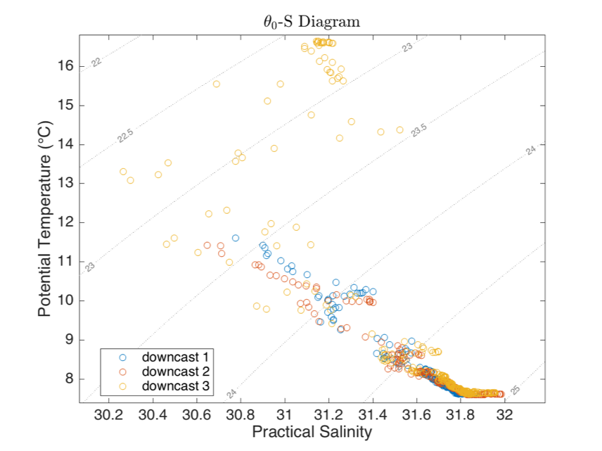
Absolute Salinity is computed internally because it is required for potential temperature and potential density. Here it is assumed that the Absolute Salinity (SA) anomaly is zero, so that SA = SR (Reference Salinity). This is probably the best approach in many coastal regions where the Absolute Salinity anomaly is not well known (see http://www.teos-10.org/pubs/TEOS-10_Primer.pdf).