RSKbinaverage.m
Input
-Required-
RSK
-Optional-
profile: [ ] (all profiles, default).direction: down (default) or up.binBy: sea pressure (default), any other channel or time.binSize: [1] (default, units of binBy)boundary: [ ] whole range (default)visualize: show plot with original and processed data on specified profile(s)
Output
RSKsamplesinbin- amount of samples in each bin
This function bins samples that fall within an interval and averages them, it is a form of data quantization.
The bins are specified using two arguments: binSize and boundary.
binSizeis the width (in units ofbinBychannel; i.e., meters if binned by depth) for each averaged bin. Typically thebinSizeshould be a denominator of the space between boundaries, but if this is not the case, the new regime will start at the next boundary even if the last bin of the current regime is smaller than the determinedbinSize.boundarydetermines the transition from onebinSizeto the next.
The cast direction establishes the bin boundaries and sizes. If the direction is up, the first boundary and binSize is closest to the seabed with the next boundaries following in descending order If the direction is down the first boundary and bin size is closest to the surface with the next boundaries following in descending order.
The boundary takes precedence over the bin size. (Ex. boundary= [5 20], binSize = [10 20]. The bin array will be [5 15 20 40 60...]).
The default binSize is 1 dbar and the boundary is between minimum (rounded down) and maximum (rounded up) sea pressure, i.e, [min(sea pressure) max(sea pressure)].
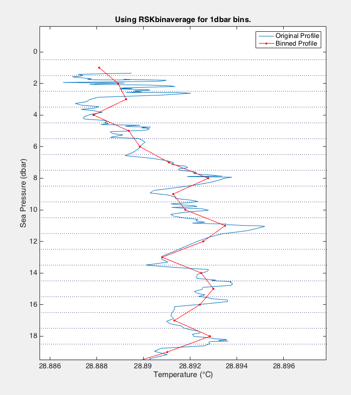
A common bining system is to use 1dbar bins from 0.5 dbar to the maximum sea pressure value. Here is the code and a diagram:
rsk = RSKbinaverage(rsk, 'direction', 'down', 'binSize', 1, 'boundary', 0.5);
|
|---|
The figure above shows an original Temperature time series plotted against Sea Pressure in blue. |
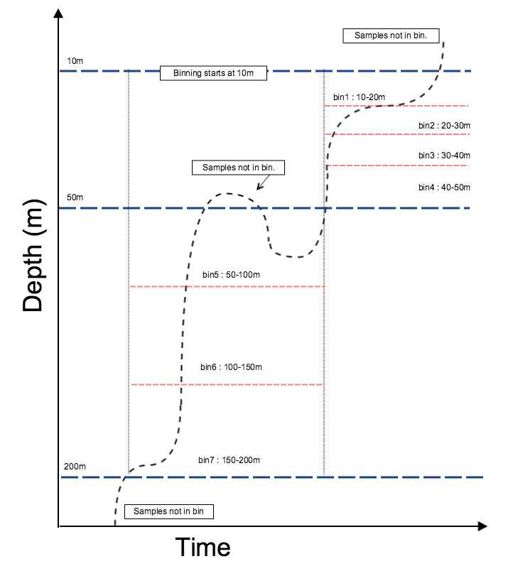
The diagram and code below describe the bin array for a more complex binning with different regimes throughout the water column:
[rsk, samplesinbin] = RSKbinaverage(rsk, 'direction', 'down', 'binBy', 'Depth', 'binSize', [10 50], 'boundary', [10 50 200])
|
|---|
| Note the discarded measurements in the image above the 50m dashed line. Once the samples have started in the next bin, the previous bin closes, and further samples in that bin are discarded. |
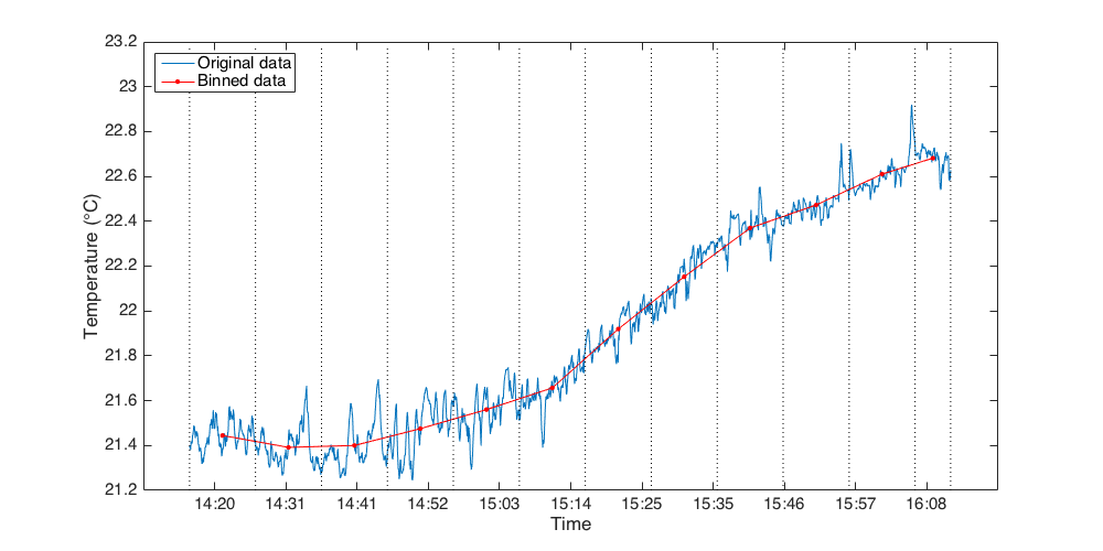
The diagram and code below gives an example when the average is done against time (i.e. binBy = 'time'), with unit in seconds. Here we average for every ten minutes (i.e. 600 seconds).
[rsk, samplesinbin] = RSKbinaverage(rsk, 'binBy', 'Time', 'binSize', 600);
|
|---|
The figure above shows an original Temperature time series plotted against Time in blue. |