Integrating with a profiling float

Introduction

There are a number of dedicated features in the RBRargo products aimed at profiling floats. The primary requirement of these vehicles is to have multiple sampling regimes that are enabled according to depth.

The typical Argo profiler might be set up with the following behaviour.

Buoyancy control

When operated on a float, the RBR instrument is used mostly as a depth sensor, providing input to the buoyancy engine and float controller. This is typically done interactively using the poll command, which can be performed at any time, regardless of whether the RBR instrument logging schedule is enabled or not. The RBR will automatically fall asleep after an idle timeout of a few seconds, but in order to minimize the power consumption, it is recommended that the command poll channellist=pressure_00 is used. This will override the idle timeouts and does not affect any ongoing deployment. It will also ensure, that the instrument is minimizing the power requirements by just powering and sampling the pressure sensor.

Always ensure the instrument is awake before sending the poll command by following the recommended wake-up procedure.

Regime sampling mode

The real science of the Argo profiler occurs during the upcast of the float, typically from 2000dbar to the surface. For historical and scientific reasons, this is often a multi-stage ascent, where the sampling and binning requirements change according to depth. The expanded figure below shows an example of a typical ascent setup for a 500dbar profile.

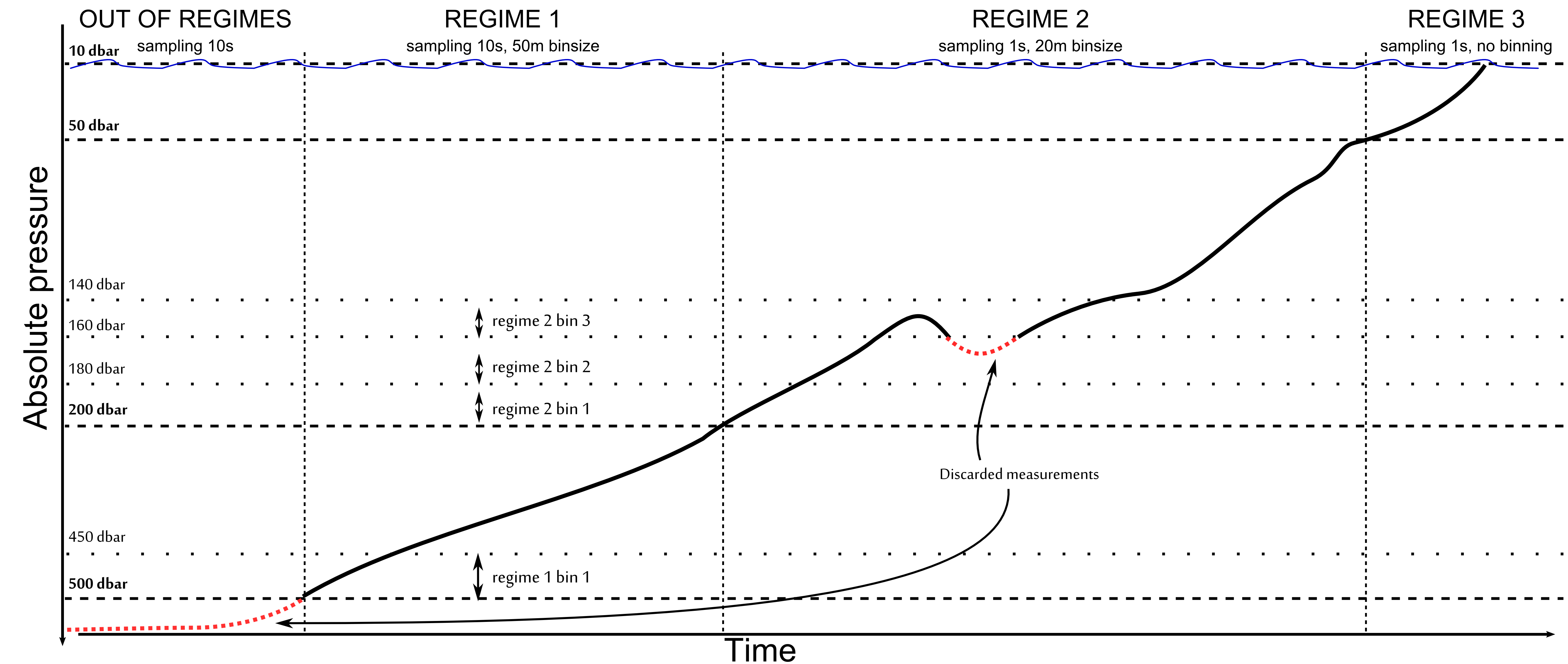
As shown above, three distinct sampling regimes are required. Each has a boundary, a sampling speed, and an averaging bin size.

The boundary determines when the regime comes into effect (dbar).
The sampling speed dictates the internal measurement rate (msec).
The bin size dictates the amount of water column (in dbar) over which the samples will be averaged and stored.

Unlike other CTDs, RBR instruments can sample through surface waters without concerns. In fact, measuring conductivity in the air can provide a reference drift measurement and a potentially useful barometric pressure reading as well.

The following chapters are various examples of how to operate the RBRargo.

Single schedule, single configuration RBRargo C.T.D example

The following is a concrete example of how to operate an RBRargo C.T.D using the regime sampling mode and how to enable/disable/download the data.

Some systems rely on instruments streaming data rather than storing it. The stream and storage parameters of the schedule command can accomplish this.

The RBRargo C.T.D is configured to collect measurements during the ascent phase:

Salinity, temperature, and absolute pressure sampled
- 0.1Hz binned 50dbar between 500dbar and 200dbar
- 1Hz binned 20dbar between 200dbar and 50dbar
- 1Hz non-binned from 50dbar to the surface

Beginning of mission, initial configuration

Ensuring default state

TEXT

>> disable
<< disable state=disabled 

>> dataset delete all
<< dataset delete all 

>> config delete all
<< config delete all 

>> schedule delete all                 
<< schedule delete all 

>> group delete all                 
<< group delete all

Group definition

In this example, only an RBRargo³ C.T.D is available on the float. The float will acquire and transmit the pressure, the salinity (with dynamic correction) and the temperature:

TEXT

>> group create gr_pts 
<< group create gr_pts
>> group gr_pts channellist=seapressure_00|salinitydyncorr_00|temperature_00
<< group gr_pts channellist=seapressure_00|salinitydyncorr_00|temperature_00

Schedule definition

The following schedule definition follows the example above (see diagram).

TEXT

>> schedule create sch_asc_pts
<< schedule create sch_asc_pts
>> schedule sch_asc_pts grouplist=gr_pts stream=off storage=on mode=regimes
<< schedule sch_asc_pts grouplist=gr_pts stream=off storage=on mode=regimes 
>> schedule sch_asc_pts direction=ascending count=3 reference=seapressure_00 finalboundary=0 boundary1=500 binsize1=50 period1=10000 boundary2=200 binsize2=20 period2=1000 boundary3=50 binsize3=0 period3=1000
<< schedule sch_asc_pts direction=ascending count=3 reference=seapressure_00 finalboundary=0 boundary1=500 binsize1=50.0 period1=10000 boundary2=200 binsize2=20.0 period2=1000 boundary3=50 binsize3=0.0 period3=1000

Configuration definition

TEXT

>> config create cf_ascent
<< config create cf_ascent
>> config cf_ascent schedulelist=sch_asc_pts
<< config cf_ascent schedulelist=sch_asc_pts

Deployment parameters

Ensure the deployment gate condition is set to none to ensure sample acquisition is entirely based on the sampling mode:

TEXT

>> deployment gate=none
<< deployment gate=none

Start of ascent

Ensures the memory is cleared first:

TEXT

>> dataset delete all
<< dataset delete all

Enable the instrument:

TEXT

>> enable config=cf_ascent dataset=ds_ascent
<< enable config=cf_ascent dataset=ds_ascent storagemode=normal state=enabled

End of ascent, disable logging and download data

Downloading the data from the instrument can be done while a schedule is still enabled (i.e. when the float is ascending), but this requires careful housekeeping to keep track of what data has been added to the dataset since the last retrieval. In this example, the logger is stopped before the download commences.

Stop the current deployment:

TEXT

>> disable
<< disable state=disabled

Determine how much memory has been used:

TEXT

>> dataset ds_ascent/sch_asc_pts/data bytecount
<< dataset ds_ascent/sch_asc_pts/data bytecount=3501260

Now loop over the data to download it in chunks:

TEXT

>> download ds_ascent/sch_asc_pts/data bytecount=<chunk-size> bytestart=0
<< download ds_ascent/sch_asc_pts/data bytecount=<chunk-size> bytestart=0<cr><lf> <bytes[start…bytecount]-of-data><crc> 

>> download
<< download ds_ascent/sch_asc_pts/data bytecount=<chunk-size> bytestart=<1 × chunk-size><cr><lf> <bytes[start…bytecount]-of-data><crc> 

>> download
<< download ds_ascent/sch_asc_pts/data bytecount=<chunk-size> bytestart=<2 × chunk-size><cr><lf> <bytes[start…bytecount]-of-data><crc>  
...
...
>> download
<< download ds_ascent/sch_asc_pts/data bytecount=<final-chunk-size> bytestart= <(n - 1) × chunk-size><cr><lf> <bytes[start…bytecount]-of-data><crc>

The data returned by the download command has a CRC value at the end. This can be used to verify the integrity of the download, but should not be stored. All chunks should be concatenated together.

Parsing the resultant data block can be done according to the description in the Sample data storage format section. Briefly, each record consists of an unsigned, 8-byte/64-bit integer timestamp and a 4-byte IEEE 754 floating-point number value for each channel.

RBRargo BGC with multiple schedules and different configurations

In the context of a BGC Argo float with many sensors, having different schedules for each sensor helps save power and can dramatically increase the lifetime of the float. This is easily achieved with the instrument by configuring multiple groups/schedules.

Here is a concrete example of an Argo BGC float configuration.

During ascending:

Salinity, temperature, and pressure sampled
- 1Hz binned 10dbar between 2000dbar and 1000dbar
- 1Hz binned 1dbar between 1000dbar and 50dbar
- 1Hz non-binned between 50dbar and 0dbar
ODO concentration, ODO temperature sampled
- 20s binned 10dbar between 1000dbar and 250dbar
- 5s binned 2dbar between 250dbar and 0dbar
pH
- 500s non-binned between 1000dbar and 250dbar
- 20s non-binned 250dbar and 0dbar
BBP700/Chlorophyll/FDOM
- 10s binned 10dbar between 2000dbar and 250dbar
- 5s binned 2dbar between 250dbar and 0dbar
Downwelling PAR and irradiance at 412nm, at 443nm, at 490nm
- 5s binned 2dbar between 250dbar and 0dbar

During park:

Salinity, temperature, pressure
- continuous every 6h
ODO concentration, ODO temperature
- continuous every 12h

When using one channel on one schedule and the same channel (or one of its supporting channels) on another schedule, their sampling frequency should be multiple. See schedule command for more details.

Beginning of the mission, initial configuration

Ensuring default state

TEXT

>> disable
<< disable status=disabled 

>> dataset delete all
<< dataset delete all

>> config delete all
<< config delete all

>> schedule delete all  
<< schedule delete all

>> group delete all
<< group delete all

Group definitions

PTS group

TEXT

>> group create gr_pts
<< group create gr_pts
>> group gr_pts channellist=seapressure_00|salinitydyncorr_00|temperature_00
<< group gr_pts channellist=seapressure_00|salinitydyncorr_00|temperature_00

ODO group

TEXT

>> group create gr_odo 
<< group create gr_odo
>> group gr_odo channellist=seapressure_00|oxygenconcentration_00|odotemperature_00
<< group gr_odo channellist=seapressure_00|oxygenconcentration_00|odotemperature_00

pH group

TEXT

>> group create gr_ph
<< group create gr_ph
>> group gr_ph channellist=seapressure_00|ph_00
<< group gr_ph channellist=seapressure_00|ph_00

BBPFL group

TEXT

>> group create gr_bbpfl
<< group create gr_bbpfl
>> group gr_bbpfl channellist=seapressure_00|backscatter_00|chlorophyll_00|fdom_00
<< group gr_bbpfl channellist=seapressure_00|backscatter_00|chlorophyll_00|fdom_00

Radiometry group

TEXT

>> group create gr_radiometry 
<< group create gr_radiometry
>> group gr_radiometry channellist=seapressure_00|par_00|irradiance_00|irradiance_01|irradiance_02
<< group gr_radiometry channellist=seapressure_00|par_00|irradiance_00|irradiance_01|irradiance_02

Schedule definitions

PTS ascending schedule

TEXT

>> schedule create sch_asc_pts
<< schedule create sch_asc_pts
>> schedule sch_asc_pts grouplist=gr_pts stream=off storage=on mode=regimes
<< schedule sch_asc_pts grouplist=gr_pts stream=off storage=on mode=regimes
>> schedule sch_asc_pts direction=ascending count=3 reference=seapressure_00 finalboundary=0 boundary1=2000 binsize1=10 period1=1000 boundary2=1000 binsize2=1 period2=1000 boundary3=50 binsize3=0 period3=1000
<< schedule sch_asc_pts direction=ascending count=3 reference=seapressure_00 finalboundary=0 boundary1=2000 binsize1=10.0 period1=1000 boundary2=1000 binsize2=1.0 period2=1000 boundary3=50 binsize3=0.0 period3=1000

ODO ascending schedule

TEXT

>> schedule create sch_asc_odo
<< schedule create sch_asc_odo
>> schedule sch_asc_odo grouplist=gr_odo stream=off storage=on mode=regimes
<< schedule sch_asc_odo grouplist=gr_odo stream=off storage=on mode=regimes
>> schedule sch_asc_odo direction=ascending count=2 reference=seapressure_00 finalboundary=0 boundary1=1000 binsize1=10 period1=20000 boundary2=250 binsize2=2 period2=5000
<< schedule sch_asc_odo direction=ascending count=2 reference=seapressure_00 finalboundary=0 boundary1=1000 binsize1=10.0 period1=20000 boundary2=250 binsize2=2.0 period2=5000

pH ascending schedule

TEXT

>> schedule create sch_asc_ph
<< schedule create sch_asc_ph
>> schedule sch_asc_ph grouplist=gr_ph stream=off storage=on mode=regimes
<< schedule sch_asc_ph grouplist=gr_ph stream=off storage=on mode=regimes
>> schedule sch_asc_ph direction=ascending count=2 reference=seapressure_00 finalboundary=0 boundary1=1000 binsize1=0 period1=500000 boundary2=250 binsize2=0 period2=20000
<< schedule sch_asc_ph direction=ascending count=2 reference=seapressure_00 finalboundary=0 boundary1=1000 binsize1=0.0 period1=500000 boundary2=250 binsize2=0.0 period2=20000

BBPFL ascending schedule

TEXT

>> schedule create sch_asc_bbpfl
<< schedule create sch_asc_bbpfl
>> schedule sch_asc_bbpfl grouplist=gr_bbpfl stream=off storage=on mode=regimes
<< schedule sch_asc_bbpfl grouplist=gr_bbpfl stream=off storage=on mode=regimes
>> schedule sch_asc_bbpfl direction=ascending count=2 reference=seapressure_00 finalboundary=0 boundary1=2000 binsize1=10 period1=10000 boundary2=250 binsize2=2 period2=5000
<< schedule sch_asc_bbpfl direction=ascending count=2 reference=seapressure_00 finalboundary=0 boundary1=2000 binsize1=10.0 period1=10000 boundary2=250 binsize2=2.0 period2=5000

Radiometry ascending schedule

TEXT

>> schedule create sch_asc_radiometry
<< schedule create sch_asc_radiometry
>> schedule sch_asc_radiometry grouplist=gr_radiometry stream=off storage=on mode=regimes
<< schedule sch_asc_radiometry grouplist=gr_radiometry stream=off storage=on mode=regimes
>> schedule sch_asc_radiometry direction=ascending count=1 reference=seapressure_00 finalboundary=0 boundary1=250 binsize1=2 period1=5000
<< schedule sch_asc_radiometry direction=ascending count=1 reference=seapressure_00 finalboundary=0 boundary1=250 binsize1=2.0 period1=5000

PTS park schedule

TEXT

>> schedule create sch_park_pts
<< schedule create sch_park_pts
>> schedule sch_park_pts grouplist=gr_pts stream=off storage=on mode=continuous period=21600000 castdetection=off
<< schedule sch_park_pts grouplist=gr_pts stream=off storage=on mode=continuous period=21600000 castdetection=off

ODO park schedule

TEXT

>> schedule create sch_park_odo
<< schedule create sch_park_odo
>> schedule sch_park_odo grouplist=gr_odo stream=off storage=on mode=continuous period=43200000 castdetection=off
<< schedule sch_park_odo grouplist=gr_odo stream=off storage=on mode=continuous period=43200000 castdetection=off

Configuration definitions

Ascent configuration

TEXT

>> config create cf_ascent
<< config create cf_ascent
>> config cf_ascent schedulelist=sch_asc_pts|sch_asc_odo|sch_asc_ph|sch_asc_bbpfl|sch_asc_radiometry
<< config cf_ascent schedulelist=sch_asc_pts|sch_asc_odo|sch_asc_ph|sch_asc_bbpfl|sch_asc_radiometry

Park configuration

TEXT

>> config create cf_park
<< config create cf_park
>> config cf_park schedulelist=sch_park_pts|sch_park_odo
<< config cf_park schedulelist=sch_park_pts|sch_park_odo

Deployment parameters

Ensure the deployment gate condition is set to none to ensure sample acquisition is entirely based on the sampling mode:

TEXT

>> deployment gate=none
<< deployment gate=none

Ascent mode

Just before ascent, enable the instrument in the ascent configuration:

TEXT

>> enable config=cf_ascent dataset=ds_ascent
<< enable config=cf_ascent dataset=ds_ascent storagemode=normal state=enabled

End of ascent

Disable the ongoing deployment:

TEXT

>> disable
<< disable state=disabled

Read info about available datasets:

TEXT

<< dataset list
>> dataset list=ds_ascent

>> dataset ds_ascent status schedulelist
<< dataset ds_ascent status=closed schedulelist=sch_asc_pts|sch_asc_odo|sch_asc_ph|sch_asc_bbpfl|sch_asc_radiometry

Get data bytecount for each schedule. Take the first schedule as an example:

TEXT

<< dataset ds_ascent/sch_asc_pts/data
>> dataset ds_ascent/sch_asc_pts/data bytecount=123456 samplecount=6172 datatype=float32

Download the PTS data by looping over the data to download it in chunks:

TEXT

>> download ds_ascent/sch_asc_pts/data bytecount=1024 bytestart=0
<< download ds_ascent/sch_asc_pts/data bytecount=1024 bytestart=0<cr><lf><1024bytes><crc>

<< download
>> download ds_ascent/sch_asc_pts/data bytecount=1024 bytestart=1024<cr><lf><1024bytes><crc>
....
<< download
>> download ds_ascent/sch_asc_pts/data bytecount=560 bytestart=122880<cr><lf><560bytes><crc>

Download the ODO data by looping over the data to download it in chunks:

TEXT

>> download ds_ascent/sch_asc_odo/data bytecount=1024 bytestart=0
<< download ds_ascent/sch_asc_odo/data bytecount=1024 bytestart=0<cr><lf><1024bytes><crc>

<< download
>> download ds_ascent/sch_asc_odo/data bytecount=1024 bytestart=1024<cr><lf><1024bytes><crc>
....
<< download
>> download ds_ascent/sch_asc_odo/data bytecount=420 bytestart=6144<cr><lf><420bytes><crc>

Download pH, BBPFL, and radiometry data in the same way.

RBRargo introspection

The list of channels populated onto an instrument and used by a float controller is subject to change depending on the float model (for example, some floats rely on hydrostatic pressure, others on absolute pressure) and the RBRargo model (e.g. an RBRargo C.T.D vs an RBRargo C.T.D.ODO).

The following list is the available channels populated for an RBRargo C.T.D.

Channel label	Description
conductivity_00	Conductivity (mS/cm)
temperature_00	Marine temperature (°C)
pressure_00	Absolute pressure (dbar) (at surface will read around 10 dbar)
seapressure_00	Hydrostatic pressure (dbar) (at surface will read around 0 dbar)
salinity_00	Salinity without dynamic correction applied (PSU)
conductivitycelltemperature_00	Internal temperature of the conductivity cell (°C)
temperaturedyncorr_00	Marine temperature corrected for C-T lag (°C)
salinitydyncorr_00	Salinity with dynamic correction applied (PSU)
cnt_00	Counts, number of sample used to calculate a bin average, when not binning, this is reporting the value 1

A complete list of possible labels is provided in the section Channel labels.

For platforms handling different models of the RBRargo, it is possible to determine the available channels by just issuing the channels command:

TEXT

>> channel list 
<< channel list=conductivity_00|temperature_00|pressure_00|sea_pressure_00|salinity_00|conductivitycelltemperature_00|temperaturedyncorr_00|salinitydyncorr_00|cnt_00

Providing platform details to end-users

Some end-users want to keep the history of the sensor's details (for example, the pressure sensor model). RBR Ltd. maintains a database of all instruments produced and their associated sensor. Providing the serial number (id command) should be sufficient in practice. However, some end users might want to have all possible information readily available from the log files sent by the float to the shore.
The instrument dumpcommand outputs the result of all the other possible commands. If the output of that command is too large to be handled by the host, RBR recommends including the results from the calibration, sensor, id, and instrument commands in the log files.

Sensor drift monitoring at the surface

It is possible to partly monitor the drift of different sensors when the float is at the surface, and sensors are exposed to air. Pressure measurements at the surface give a direct offset correction:

CODE

>> calibration pressure_00 datetime=20240501140000 offset=0.2
<< calibration pressure_00 datetime=20240501140000 offset=200.00000e-3

Optical dissolved oxygen measurements in the air will also provide a reference for drift correction (see published literature). Measuring conductivity at the surface not only gives the opportunity to confirm that the float is effectively at the surface but also allows the monitoring of any electronic drift in the conductivity, as the sensor should read around 0. Conductivity in air measurements needs to be taken with precaution. It is advised to acquire several measurements in air and not just one, as waves might wash the conductivity cell. If only one conductivity value is to be transmitted to shore, always use the lowest value. If possible, it is preferable to report directly the conductivity and not the salinity as the PSS78 calculation will saturate at 0 (see pss78 - derivation of Practical Salinity (1978)).

Energy tracking

The instrument tracks energy consumed via the command instrument power external.