Integrating with a profiling float

Introduction

There are a number of dedicated features in the RBR L3 products aimed at profiling floats. The primary requirement of these vehicles is to have multiple sampling regimes that are enabled according to depth.

The typical Argo profiler might be set up with the following behaviour:

Buoyancy control

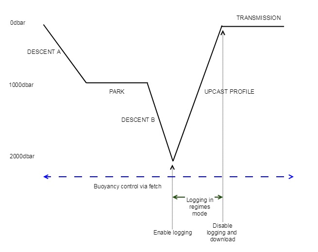
For the majority of this 10-day schedule, the RBR instrument is used purely as a depth sensor, providing input to the buoyancy engine and float controller. This is typically done interactively using the fetch command, which can be performed at any time, regardless of whether the RBR instrument logging schedule is enabled or not. The RBR will automatically fall asleep after an idle timeout of a few seconds, but in order to minimize the power consumption, it is recommended that the command fetch sleepafter = true, channels = pressure_00 is used. This will override the idle timeouts and does not affect any ongoing deployment. It will also ensure, that the instrument is minimizing the power requirements by just powering and sampling the pressure sensor.

Always ensure the instrument is awake before sending the fetch by following the recommended wake-up procedure.

Setup for ascent, enable logging

The real science of the Argo profiler occurs during the upcast, typically from 2000dbar to the surface. For historical and scientific reasons, this is often a multi-stage ascent, where the sampling and binning requirements change according to depth. The expanded figure below shows an example of a typical ascent setup.

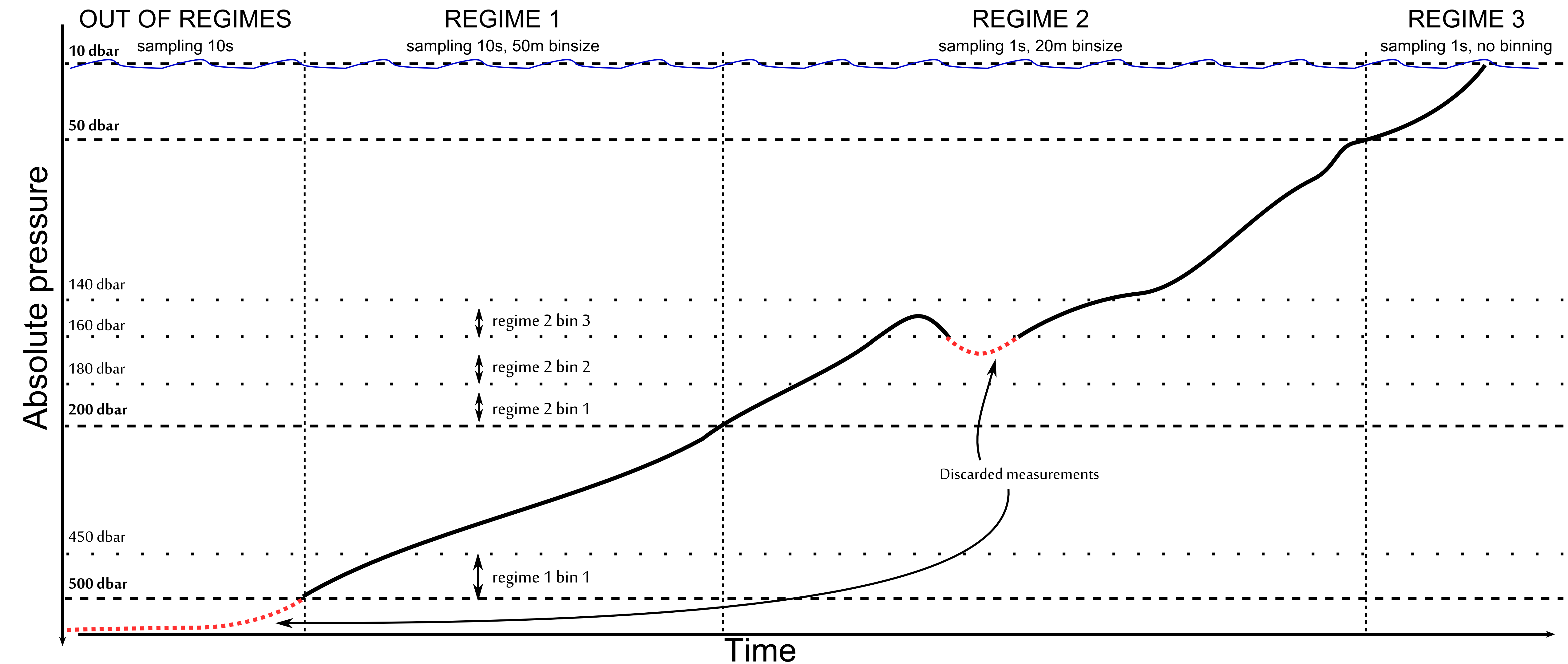
As is clear, there are three distinct sampling regimes that are required. Each of them has a boundary, a sampling speed, and an averaging bin size.

• The boundary determines when the regime comes into effect (dbar).
• The sampling speed dictates the measurement rate that is used internally (msec).
• The bin size dictates the amount of water column (in dbar) over which the samples will be averaged and stored.

To accomplish this task, a combination of the regimes and three regime commands are needed.

First, one should tell the logger that it will be ascending (decreasing water pressure) using three sampling regimes, and the absolute pressure serves as reference.

Configure the regime closest to the seabed (10s sampling rate, 50m bin, bottom boundary 500 dbar):Then the middle one (1s sampling rate, 20m bin, bottom boundary 200 dbar):Then the regime closest to the sea surface (1s sampling rate, no binning, bottom boundary 50 dbar):Finally put the logger in regimes mode:With this setup, the logger will only start recording data once the boundary of the first regime is crossed. In this example, if the RBR instrument is enabled while the float is at 700 dbar, then starts to ascend, no data will be stored until 500 dbar. If the float is at 490 dbar when the RBR instrument is enabled, sampling will start immediately as the first regime is already in effect.

Instruments can be shipped with a derived data channel populated, type cnt_00 , which contains a count of the number of measurements in the averaged bin when in the regimes sampling mode. As with any other channel, it may be turned on or off as needed; see the channel command. The benefit of turning it on when storing data in EasyParse format is that the value is then available when the main sample data in dataset-1 is downloaded. Otherwise, the dataset containing the events must also be retrieved if these values are needed.

Ensure the logger will use the EasyParse format (calbin00).

Starts the logger while ensuring the memory is cleared first.There will also be a bin in progress which never completes, once the float has risen to the surface. However, issuing the stop command will flush the final bin to memory, regardless of whether it is complete or not.

End of ascent, disable logging and download data

Downloading the data from the instrument can be done while a schedule is still enabled, but this requires careful housekeeping to keep track of what data has been added to the dataset since the last retrieval. In this example, the logger is stopped before the download commences.

Stop the current deployment

Determine how much memory has been used:Now loop over the data to download it in chunks:The data returned by the read command has a CRC value at the end. This can be used to verify the integrity of the download, but should not be stored. All chunks should be concatenated together.

Parsing the resultant data block can be done according to the description in the "EasyParse format" section Briefly, each record consists of an unsigned, 8-byte/64-bit integer timestamp, and a 4-byte IEEE 754 floating-point number value for each channel.

More details on the calculation

Please note that samples taken in a bin where the outer limit has previously been exceeded are discarded, as shown in the example figure.

Available output channels

The list of channels populated onto an instrument and enabled by a float controller is subject to change depending on the float model (for example, some floats rely on hydrostatic pressure, others on absolute pressure) or revision (dynamic correction channels available only since fw 1.146). 

Post-processing onboard

Starting from firmware 1.135, it is possible to bin the data after the ascent and to generate more statistics (like the standard deviation of samples) via the postprocessing command. The regimes mode is still relevant in conjunction with post-processing to retain a different sampling rate, but with the parameter binsize set to 0 to record all samples as the postprocessing command relies on data stored in dataset-1 to generate post-processed data. 

At the end of the ascent, stop logging, and wait for the post-processing to finish:

And download the post-processed data (dataset-4):

Providing platform details to end-users

Some end-users want to keep the history of the sensor's details (for example, pressure sensor model). RBR Ltd. maintains a database of all instruments produced and their associated sensor. Providing the serial number (id command) should be sufficient in practice. But some end users might want to have all possible information readily available from the log files sent by the float to the shore.
The getall command outputs the result of all the other possible commands. If the output of that command is too large to be handled by the host, RBR recommends including the results from the calibration, sensor, id, and info commands in the log files.

Sensor drift monitoring at surface

It is possible to partly monitor the drift of different sensors when the float is at the surface and sensors are exposed to air. Pressure measurements at the surface give a direct offset correction. Optical dissolved oxygen measurements, air measurements, will also provide a reference for drift correction (see published literature). Measuring conductivity at the surface not only gives the opportunity to confirm that the float is effectively at the surface but also allows to monitor any electronic drift in the conductivity as the sensor should read around 0. Conductivity in air measurements needs to be taken with precaution. It is advised to acquire several measurements in air and not just one as the conductivity cell might be washed by waves. If only one conductivity value is to be transmitted to shore, always use the lowest value. It is preferable to report directly the conductivity and not the salinity as the PSS78 calculation will saturate at 0 (see Example 7: pss78 - derivation of Practical Salinity (1978)).

Energy tracking

The instrument allows to track energy consumed via the command powerexternal .